Properly Requesting Reaction Forces in Abaqus

What are Reaction Forces?

Reaction forces are exerted by a body when an external force is being applied to it. For instance, if you’re walking on the street, there will be a resultant reaction force exerted by the street. This reaction force has two components. First, we have a vertical component to support the force from your weight. The second is a tangential component, friction. And so, from this example, it becomes apparent that those forces are only present at constrained nodes, and not free ones. This is also where Abaqus calculates reaction forces.

Let’s take a look at two ways to find and plot the reaction forces, as well as why you might choose one over the other.

Model Setup

The model below shows an explicit simulation of a rigid sphere bouncing on a trampoline. We’ve modeled the trampoline bed as well as the trampoline frame using S4 elements. As for the sphere, we’re using R3D4 elements. Lastly, we’ve modeled the springs as SPRINGA elements.

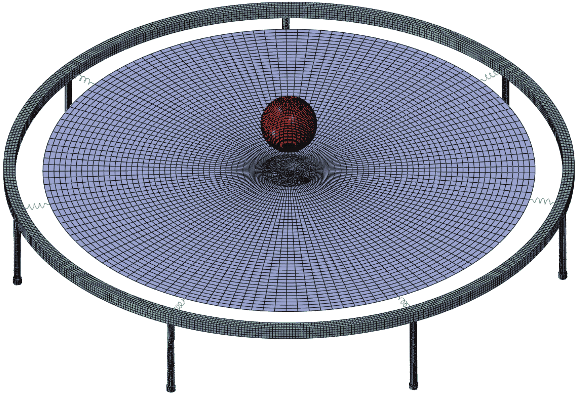
The legs of the trampoline frame are fixed in all degrees of freedom (ENCASTERED). Additionally, the bases of all seven legs of the frame are tied to a reference point using a kinematic coupling constraint. Since this is a drop test, we’ll apply an initial velocity of 5 m/s to the rigid sphere. A gif shows an animation of the simulation, with the color field set to von Mises stress.

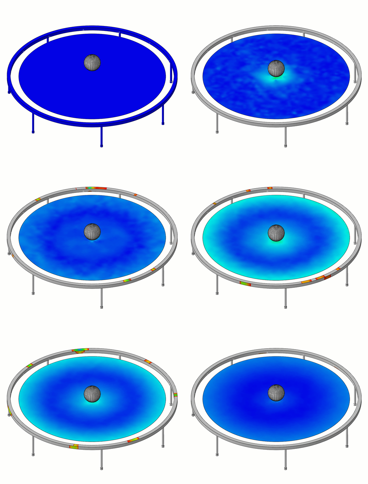
Because the legs of the frame are constrained in all degrees of freedom, Abaqus will calculate the reaction forces there, and only there.

There are two ways of extracting the reaction force:

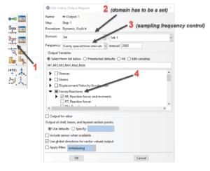
1. To obtain the data at better resolution with a higher sampling rate, you can request the reaction force history output at the reference point tied to the legs. You can adjust the frequency to output at higher sampling rates.
   • In Abaqus/CAE, this is done by Output > History Output Requests > Create, then choosing RF under Forces/Reactions
   • In the input file:

     *Output, history, time interval=0.0005
     
     *Node Output, nset=Set-1
     
     RF1, RF2, RF3, RM1, RM2, RM3

     (Set-1 contains the reference point mentioned earlier)

     

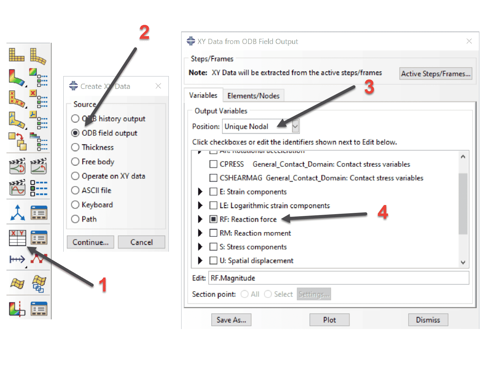
2. If you forget to request the history output, Abaqus, by default, outputs preselected field output variables. After step 4 (below), be sure to select the reference node tied to the legs of the trampoline frame. You can find this under the Elements/Nodes tab.

Plotting Reaction Forces Results and Discussion

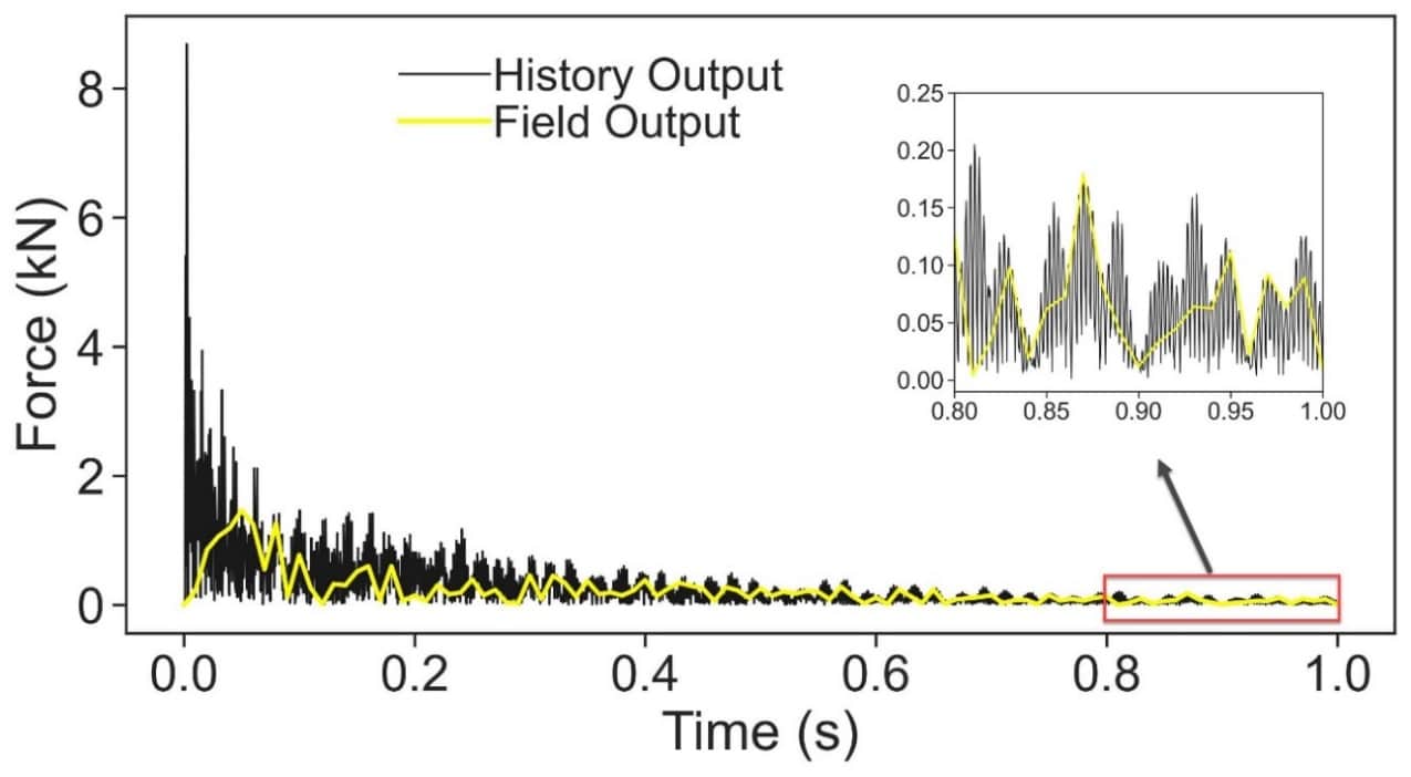
To highlight the difference between the two methods of obtaining the reaction force, I’ve overlaid the reaction force from the history output as well as that from the field output in one plot. This plot shows the force on the legs of the frame obtained from the history output. The period is 0.0005 seconds, or a sampling frequency of 2000 Hz, resulting in 2000 points. Additionally, you’ll see the same force obtained at a much lower sampling frequency from the field output variable, shown in yellow.

Within the range of 0.8 s to 1 s, it is clear that the force from the history output is well sampled, while the force obtained from the field output is under-sampled and does not represent the complete behavior of the structure.

Capturing the reaction force at a high sampling rate is typically only a concern for high dynamic systems. This is not the case when using Abaqus/Standard to run static analyses. For such studies, it’s sufficient to observe the reaction force coming from the field output, as the last increment is what matters.

Conclusion

To summarize, I would advise you to always output reaction forces using the history output rather than the field output. Depending on your application, and if you want to output the reaction force at a high sampling rate, you can do this without sacrificing memory on your disk.

Bilal Abdul Halim
Application Engineer Specialist, Simulation
Computer Aided Technology